Differentials Introduction. Approximation. Newtons Method.

Published 8/16/2025
Differentials and Linear Approximation
Differentials and Linear ApproximationLet y=f(x). For a chosen step Δx, Δy:=f(x+Δx)−f(x).If f is differentiable at x, ΔxΔy→f′(x) as Δx→0, so for small stepsΔy≈f′(x)Δxand, since Δy=f(x+Δx)−f(x),f(x+Δx)≈f(x)+f′(x)ΔxThis gives a first–order (linear) way to estimate nearby values of f.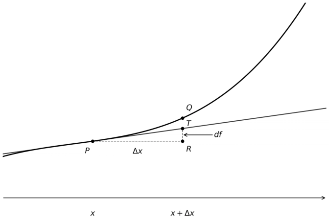
The image above depicts the df infinitesimal change (RT) on graph which approximates to the ∆y change (which is RQ) for sufficiently small "∆x" (PR) changes.
Differential viewpointFirst, name the predicted tiny change in the output as the infinitesimal symbol dy.It is not the actual finite change Δy; it records what the linear rule predicts at the point x.To compute this prediction, pair it with an infinitesimal input step dx.Think of dx as an infinitesimally small step in x (same units as x).The derivative ties them together:dy=f′(x)dxRead: slope at x× infinitesimal input step = infinitesimal predicted output step.The standard calculus terms are “linear approximation” and “linearization.”This linear prediction is the linear approximation (linearization) of f at x; its error is quadratic in Δxwhen f is sufficiently smooth (so the neglected part behaves like C(Δx)2 for small Δx).To compare with a concrete finite step Δx, take dx=Δx and get Δy≈dy=f′(x)dx.dxdy=f′(x) summarizes the proportionality of these infinitesimal symbols,whereas ΔxΔy is a finite average rate approaching f′(x) as Δx→0.A units check: if x has units U, then f′(x) has units (output)/U, so f′(x)dx has output units, matching dy.Example: approximate a cube root near 8Let f(x)=x1/3, x=8, Δx=0.3. f(8)=2,f′(x)=31x−2/3⇒f′(8)=121.Differential step: take dx=Δx=0.3, dy=f′(8)dx=121⋅0.3=0.025.Linear estimate: f(8+Δx)≈f(8)+dy=2+0.025=2.025.Here dy is the infinitesimal stand-in for the true Δy=f(8.3)−2; for a small step like 0.3 the two are close.SummaryIntroduce dy as the infinitesimal output change and dx as the paired infinitesimal input step;tie them by dy=f′(x)dx; for a chosen finite step Δx, set dx=Δx to get Δy≈dy.Newton's Method
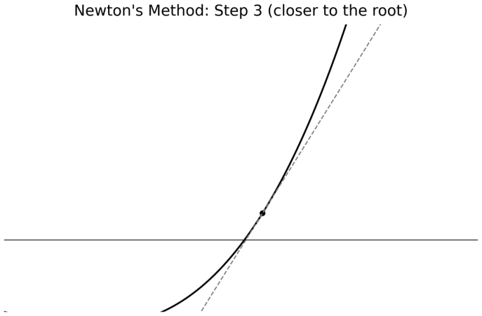
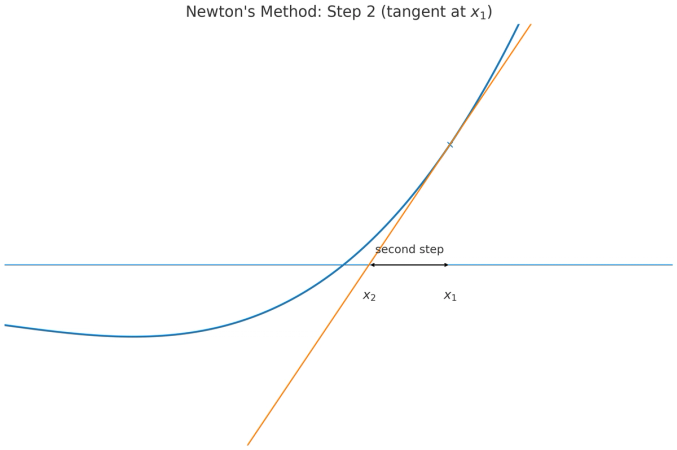
Newton’s methodWe seek a number r with f(r)=0. Starting from a provisional value x0,we replace the curve y=f(x) near x0 by its tangent line. The tangent at x0 has equationy−f(x0)=f′(x0)(x−x0).Imposing the x-axis condition y=0 gives 0−f(x0)=f′(x0)(x1−x0), hencex1=x0−f′(x0)f(x0).Repeating the same construction at x1, then at x2,and so on, yields the iterationxn+1=xn−f′(xn)f(xn).This update is precisely the solution of the linear equation f(xn)+f′(xn)(x−xn)=0,that is, the x-intercept of the tangent drawn at (xn,f(xn)).The construction is local, depending only on f near the root. If f is differentiable at a simple root r with f′(r)=0 and the start is close,the iterates converge rapidly; the tangent error is quadratic in the step.Caution: if f′(xn)=0 the step is undefined; if ∣f′(xn)∣ is small, the step may be too large. Far from a simple root the tangent may cross poorly,causing divergence.In practice one monitors ∣f(xn)∣ or ∣xn+1−xn∣ and stops at tolerance. If overshoot occurs, use damping:xn+1=xn−λf′(xn)f(xn),0<λ≤1.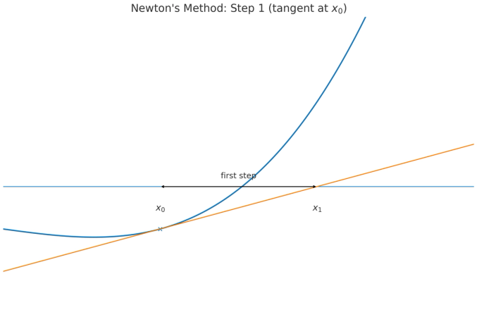
The more iterations we have passed, the closer we get to the "root" value of the function.
Example: solve ex=3 (so x=ln3).f(x)=ex−3, f′(x)=ex, x0=1.Step 1: f(x0)=e−3≈−0.281718, f′(x0)=e≈2.718282, x1=e3≈1.103638.Step 2: f(x1)=ex1−3≈0.015116, f′(x1)=ex1≈3.015116,x2=x1−f′(x1)f(x1)≈1.0986249.Step 3: x3=x2−ex2ex2−3≈1.09861229, so ln3≈1.09861229.